Simulating returns using either the traditional closed-form equations or probabilistic models similar Monte Carlo has been the touchstone practice to gibe them against empirical observations from stock, bond as well as other fiscal time-series data. (See Chan as well as Ng, 2017 as well as Lopez de Prado, 2018.) Some of the stylised facts of render distributions are equally follows:
- The tails of an empirical render distribution are ever thick, indicating lucky gains as well as enormous losses are to a greater extent than likely than a Gaussian distribution would suggest.
- Empirical distributions of assets show sudden peaks which traditional models are oft non able to gauge.
To generate simulated render distributions that are faithful to their empirical counterpart, I tried my mitt on diverse kinds of Generative Adversarial Networks, a really specialised Neural Network to larn the features of a stationary serial we’ll depict later. The GAN architectures used hither are a straight descendant of the uncomplicated GAN invented past times Goodfellow inwards his 2014 paper. The ones tried for this exercise were the conditional recurrent GAN as well as the uncomplicated GAN using fully connected layers. The thought involved inwards the architecture is that at that spot are 2 constituent neural networks. One is called the Generator which takes a vector of random dissonance equally input as well as thence generates a fourth dimension serial window of a dyad of days equally output. The other element called Discriminator tries to conduct maintain either this generated window equally input or takes a existent window of cost returns or other features equally input as well as tries to decipher whether a given window of returns or other features is “real” ( from the AAPL data) or “fake” (generated past times the Generator). The labor of the generator is to travail to “fool” the discriminator past times successively (as it is beingness trained) generating to a greater extent than “real” data. The preparation goes on until:
1) the generator is able to output the characteristic laid which is identical inwards distribution to the existent dataset on which both the networks were trained
2) The discriminator is able to state existent information from the generated one
The mathematical objectives of this preparation are to maximise:
a ) log(D(x)) + log(1 - D(G(z))) - Done past times the discriminator - Increase the expected ( over many iterations ) log probability of the Discriminator D to position betwixt the existent as well as faux samples x. Simultaneously, increase the expected log probability of discriminator D to correctly position all samples generated past times generator G using dissonance z.
b) log(D(G(z))) - Done past times the generator - So, equally observed empirically piece preparation GANs, at the outset of preparation G is an extremely pathetic “truth” generator piece D speedily becomes practiced at identifying existent data. Hence, the element log(1 - D(G(z))) saturates or remains low. It is the labor of G to maximize log(1 - D(G(z))). What that agency is G is doing a practiced labor of creating existent information that D isn’t able to “call out”. But because log(1 - D(G(z))) saturates, nosotros develop G to maximize log(D(G(z))) rather than minimize log(1 - D(G(z))).
Together the min-max game that the 2 networks play betwixt them is formally described as:
minGmaxDV (D, G) =Epdata(x)[log D(x)] +E p(z) [log(1 − D(G(z)))]
The existent information sample x is sampled from the distribution of empirical returns pdata(x)and the zis random dissonance variable sampled from a multivariate gaussian p(z). The expectations are calculated over both these distributions. This happens over multiple iterations.
The hypothesis was that the diverse GANs tried volition move able to generate a distribution of returns which are closer to the empirical distributions of returns than ubiquitous baselines similar Monte Carlo method using the Geometric Brownian motion.
The experiments
A bird’s-eye persuasion of what we’re trying to do hither is that we’re trying to larn a joint probability distribution across fourth dimension windows of all features along amongst the per centum alter inwards adjusted close. This is thence that they tin move simulated organically amongst all the nuances they naturally come upwards together with. For all the GAN preparation processes, Bayesian optimisation was used for hyperparameter tuning.
In this exercise, initially, nosotros initiatory of all collected to a greater extent than or less features belong to the categories of trend, momentum, volatility etc similar RSI, MACD, Parabolic SAR, Bollinger bands etc to do a characteristic assault the adjusted unopen of AAPL information which spanned from the 1980s to today. The window size of the sequential preparation sample was laid based on hyperparameter tuning. Apart from these indicators the per centum alter inwards the adjusted OLHCV information were taken as well as concatenated to the listing of features. Both the generator as well as discriminator were recurrent neural networks ( to sequentially conduct maintain inwards the multivariate window equally input) powered past times LSTMs which farther passed the output to dense layers. I conduct maintain tried learning the articulation distributions of xiv as well as likewise 8 features The results were suboptimal, in all likelihood because of the architecture beingness used as well as likewise because of how notoriously tough the GAN architecture mightiness move out to train. The suboptimality was inwards price of the generators’ mistake non reducing at all ( log(1 - D(G(z))) saturating really early on inwards the preparation ) after initially going upwards as well as the random render distributions without whatever item shape beingness generated past times the generators.
After trying conditional recurrent GANs, which didn’t develop well, I tried using simpler multilayer perceptrons for both Generator as well as Discriminators inwards which I passed the entire window of returns of the adjusted unopen cost of AAPL. The optimal window size was derived from hyperparameter tuning using Bayesian optimisation. The distribution generated past times the feed-forward GAN is shown inwards figure 1.
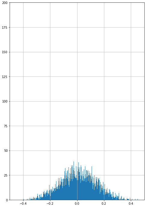
Fig 1. Returns past times uncomplicated feed-forward GAN
Some of the mutual problems I faced were either partial or consummate mode collapse - where the distribution either did non conduct maintain a similar sudden peak equally the empirical distribution ( partial ) or any noise sample input into the generator produces a express laid of output samples ( complete).
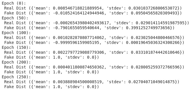
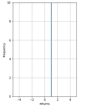
The figure higher upwards shows way collapsing during training. Every subsequent epoch of the preparation is printed amongst the hateful as well as touchstone departure of both the empirical subset (“real data”) that is position into the discriminator for preparation as well as the subset generated past times the generator ( “fake data”). As nosotros tin run across at the 150th epoch, the distribution of the generated “fake data” absolutely collapses. The hateful becomes 1.0 as well as the stdev becomes 0. What this agency is that all the dissonance samples position into the generator are producing the same output! This phenomenon is called Mode Collapse equally the frequencies of other local modes are non inline amongst the existent distribution. As you lot tin run across inwards the figure below, this is the finally distribution generated inwards the preparation iterations shown above:
A few tweaks which reduced errors for both Generator as well as Discriminator were 1) using a dissimilar learning charge per unit of measurement for both the neural networks. Informally, the discriminator learning charge per unit of measurement should move ane lodge higher than the ane for the generator. 2) Instead of using fixed labels similar 1 or a 0 (where 1 agency “real data” as well as 0 agency “fake data”) for preparation the discriminator it helps to subtract a small-scale dissonance from the label 1 as well as add together a similar small-scale dissonance to label 0. This has the termination of changing from classification to a regression model, using hateful foursquare mistake loss instead of binary cross-entropy equally the objective function. Nonetheless, these tweaks conduct maintain non eliminated completely the suboptimality as well as way collapse problems associated amongst recurrent networks.
Baseline Comparisons
We compared this generated distribution against the distribution of empirical returns as well as the distribution generated via the Geometric Brownian Motion - Monte Carlo simulations done on AAPL via python. The metrics used to compare the empirical returns from GBM-MC as well as GAN were Kullback-Leibler divergence to compare the “distance” betwixt render distributions as well as VAR measures to sympathize the hazard beingness inferred for each sort of simulation. The chains generated past times the GBM-MC tin move seen inwards fig. 4. Ten paths were simulated inwards M days inwards the time to come based on the inputs of the variance as well as hateful of the AAPL stock information from the 1980s to 2019. The input for the initial cost inwards GBM was the AAPL cost on 24-hour interval one.
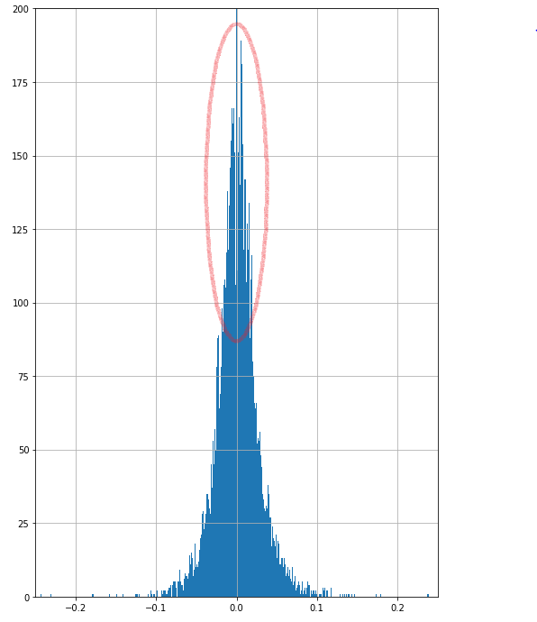
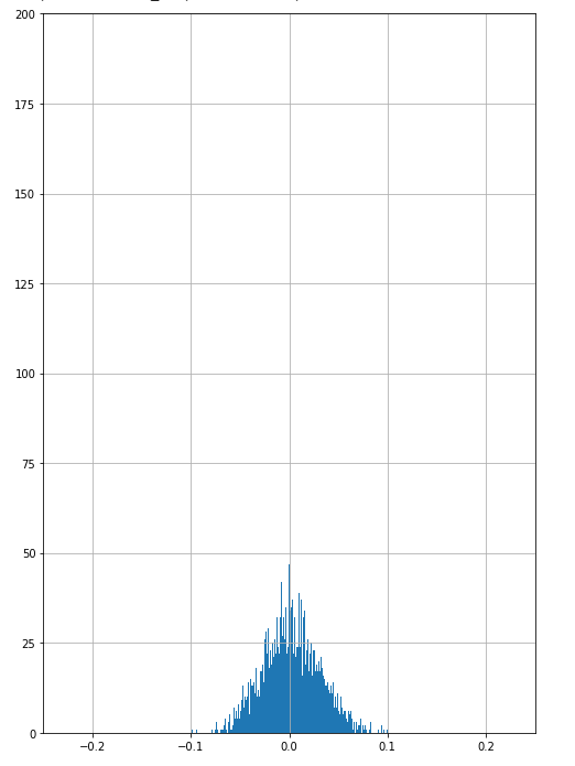
Fig 2. shows the empirical distributions for AAPL starting 1980s upwards till now. Fig 3. shows the generated returns past times Geometric Brownian motion on AAPL.
To compare the diverse distributions generated inwards the exercise I binned the render values into 10,000 bins as well as thence calculated the Divergence using the non-normalised frequency value of each bin. The code is:
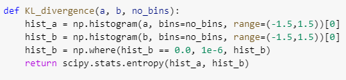
The formula scipy uses behind the scene for entropy is:
S = sum(pk * log(pk / qk)) where pk,qk are bin frequencies
The Geometric Brownian Motion generation is a ameliorate gibe for the empirical information compared to the ane generated using Multiperceptron GANs fifty-fifty though it should move noted that both are extremely bad.
The VAR values ( calculated over 8 samples ) hither state us that beyond a confidence level, the sort of returns (or losses) nosotros mightiness acquire - inwards this case, it is the per centum losses amongst 5% as well as 1% conduct a opportunity given the distributions of returns:
The GBM generator VARs appear to move much closer to the VARs of the Empirical distribution.
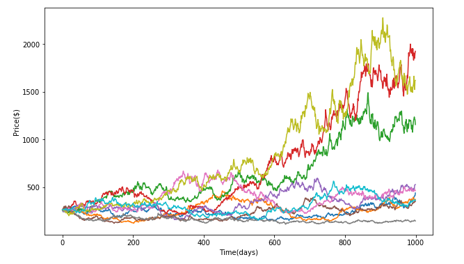
. Fig 4. Showing the diverse paths generated past times the Geometric Brownian motion model using monte Carlo.
Conclusion
The distributions generated past times both methods didn’t generate the sudden peak shown inwards the empirical distribution (figure 2). The spread of the render distribution past times the GBM amongst Monte Carlo was much closer to reality equally shown past times the VAR values as well as its distance to the empirical distribution was much closer to the empirical distribution equally shown past times the Kulback-Leibler divergence, compared to the ones generated past times the diverse GANs I tried. This exercise reinforced that GANs fifty-fifty though enticing are tough to train. While at it I discovered as well as read most a few tweaks that mightiness move helpful inwards GAN training. Some of the mutual problems I faced were 1) mode collapse discussed higher upwards 2) Another ane was the saturation of the generator as well as “overpowering” past times the discriminator. This saturation causes suboptimal learning of distribution probabilities past times the GAN. Although non actually successful, this exercise creates ambit for exploring the diverse newer GAN architectures, inwards add-on to the conditional recurrent as well as multilayer perceptron ones which I tried, as well as utilization their fabled powerfulness to larn the subtlest of distributions as well as apply them for fiscal time-series modelling. Our codes tin move industrial plant life at Github here. Any modifications to the codes that tin assist improve surgical procedure are most welcome!
About Author:
Akshay Nautiyal is a Quantitative Analyst at Quantinsti, working at the confluence of Machine Learning as well as Finance. QuantInsti is a premium institute inwards Algorithmic & amongst instructor-led as well as self-study learning programs. For example, at that spot is an interactive course on using Machine Learning inwards Finance Markets that provides hands-on preparation inwards complex concepts similar LSTM, RNN, cross validation as well as hyper parameter tuning.
Industry update
1) Cris Doloc published a novel mass “Computational Intelligence inwards Data-Driven Trading” that has extensive discussions on applying reinforcement learning to trading.
2) Nicolas Ferguson has translated the Kalman Filter codes inwards my mass Algorithmic Trading to KDB+/Q. It is available on Github. He is available for programming/consulting work.
3) Brain Stanley at QuantRocket.com wrote a weblog post on "Is Pairs Trading Still Viable?"
4) Ramon Martin started a novel weblog amongst a slice on "DeepTrading amongst Tensorflow IV".
5) Joe Marwood added my mass to his top 100 trading books list.
6) Agustin Lebron's novel mass The Laws of Trading contains a practiced interview interrogation on adverse pick (via Bayesian reasoning).
7) Linda Raschke's novel autobiography Trading Sardines is hilarious!
Tidak ada komentar:
Posting Komentar